Measuring AI Agent Latency Beyond Single-Call Benchmarks
Part 2 of 3 — The Experiments

Part 1 covered the architecture. This post covers the experiments, what two benchmark tiers showed, and why the results looked completely different depending on which one you ran.
Same GPU. Same model. One optimization enabled.
If you only ran the standard gateway-direct test, you would see identical numbers and have no reason to prefer one configuration over the other. The agent end-to-end tier is what shows the actual difference.
Quick recap from Part 1: A user query hits a proxy gateway, which routes it to a model server running on a cloud GPU. The agent doesn’t call the model once it calls it 3 to 5 times per task, with each call carrying the full conversation history. A single-call benchmark doesn’t capture any of that.
Experiment Design: Three Optimization Paths
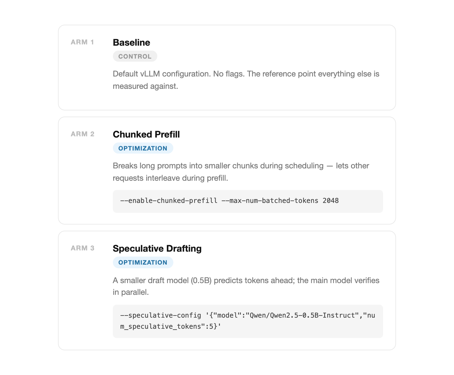
I tested three vLLM server configurations (or “arms”) on a single Lambda A10G-24GB using Qwen2.5-3B-Instruct. The goal was to isolate how different infrastructure flags handle agentic workloads.
Prompt Growth in Agentic Loops
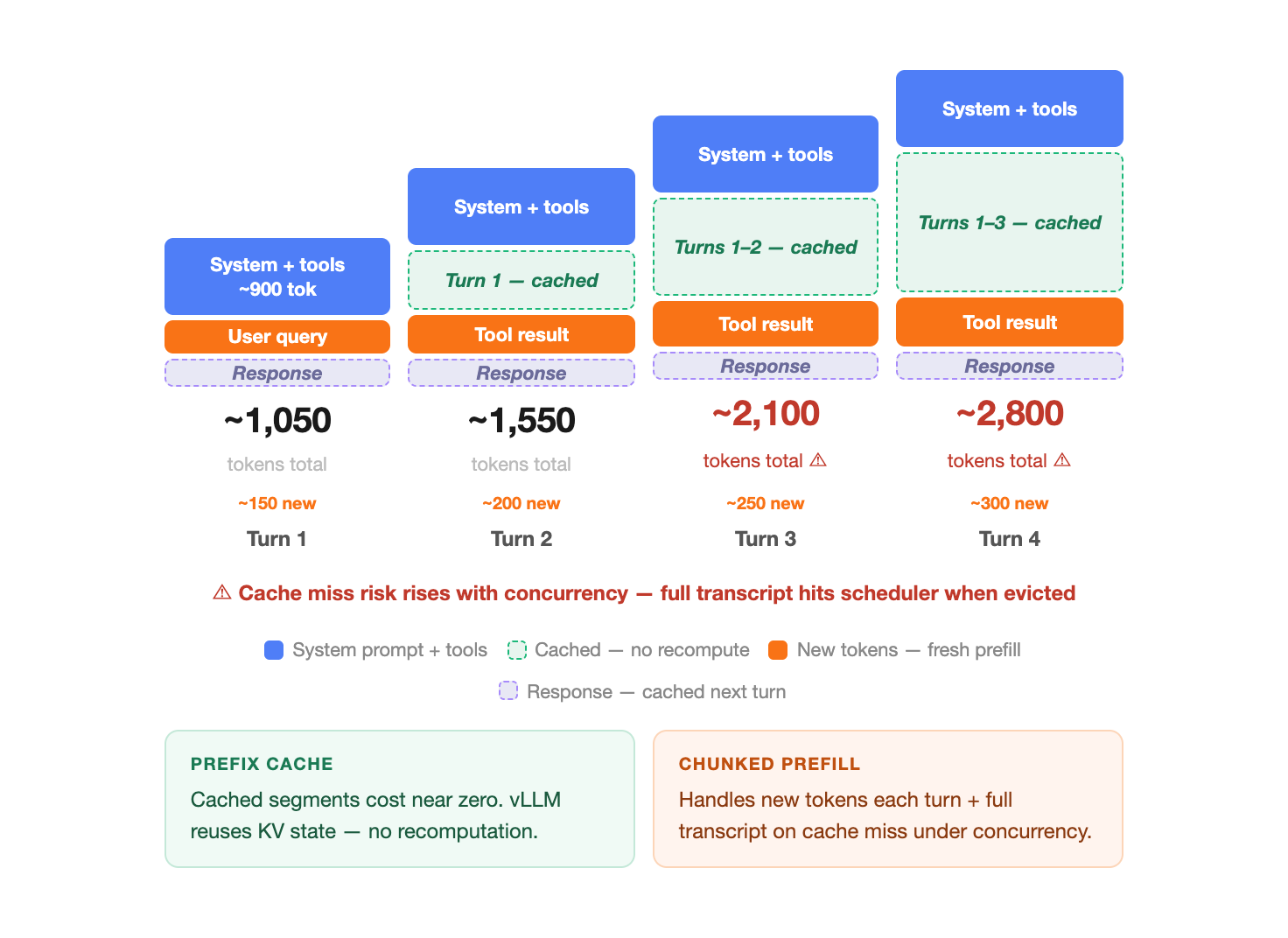
Unlike a simple chatbot, an agent maintains a running transcript of every tool call and search result. By the third turn of a conversation, the prompt often exceeds 2,000 tokens.
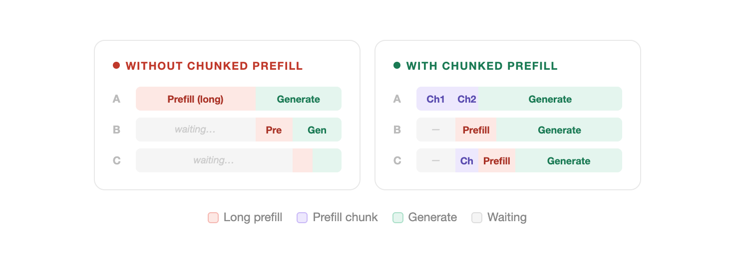
In a default setup, the GPU reads this entire 2,000-token prompt in one uninterrupted block. While it’s doing that, every other request in the system is forced to wait — a scheduling bottleneck that compounds under concurrency.
This is the same proxy-to-model path from Part 1, now under concurrent load, the growing transcript is what turns a latency problem into a scheduling problem.
Technical Context: The Prefill Phase
LLM inference happens in two stages:
Prefill: The model reads and processes the prompt. This is computationally expensive.
Generation: The model writes the response token-by-token.
Chunked prefill forces the system to process that long prompt in pieces, letting other requests run in between. This keeps concurrent requests from stalling behind a long prefill block.
Side note: Direction this points toward, separating prefill and decode onto different hardware entirely — disaggregated prefill/decode. Different phases, different GPU requirements. Worth knowing this exists if you’re thinking about where inference optimization goes next.
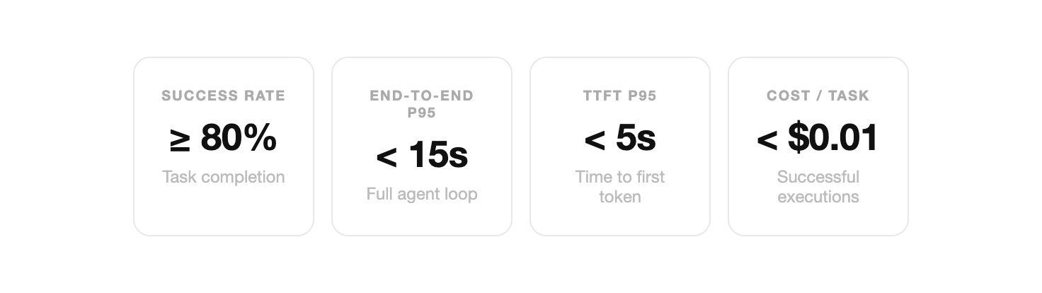
Setting Targets: SLOs and Performance Hypotheses
I defined these Service Level Objectives (SLOs) before looking at the data. An SLO written after the fact isn’t a goal — it’s just a description of what happened.
Pre-Experiment Predictions
Chunked prefill should reduce tail latency: Agents send long prompts but give short answers — exactly the scheduling pattern this flag is designed for.
Speculative decoding is unlikely to help here: It works best on predictable outputs. Agent tool-call responses are JSON with variable structure — low acceptance rates for the draft model, which adds overhead rather than saving time.
Prefix caching should activate consistently: Every agent starts with the same ~900-token system prompt. vLLM should reuse that computed result instead of recalculating it every time.
Functional Validation: The Golden Set
Speed is irrelevant if the agent is producing wrong answers. Before running load tests, I ran a “Golden Set” of 10 fixed queries to verify accuracy.
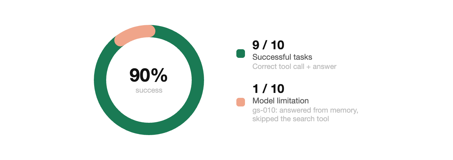
The one failure (query gs-010) was a model-level limitation where the 3B model answered from its own knowledge instead of calling the search tool.
Tiered Benchmarking: Gateway vs. End-to-End
When concurrency increased, the infrastructure differences became visible.
Tier 1: Gateway-Direct
This is what standard benchmarks measure and showing a null result here is the point, not a limitation.
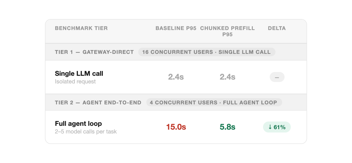
16 concurrent users each sent a single isolated call. p95 is the response time the slowest 5% of requests experience.
Finding: Baseline and Chunked Prefill were identical at 2.4s (p95).
If you stopped here, you would conclude the optimization made no difference. That conclusion would be wrong — gateway-direct measures a single isolated call, not the multi-call sequence an agent actually runs.
Tier 2: Agent End-to-End
4 concurrent users each ran full agent tasks (3–5 sequential model calls).
Finding: Baseline latency reached 15.0s, while Chunked Prefill held at 5.8s.
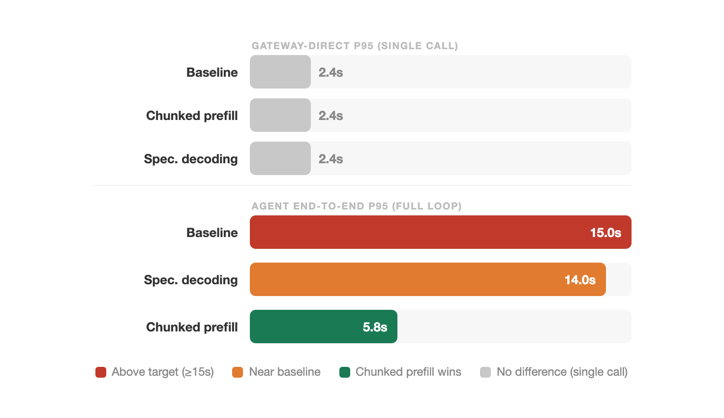
The “tail” latency the slowest 5% of requests is 3× better with chunked prefill. By forcing the scheduler to share resources in between chunks, long-prompt requests add 9+ seconds of tail latency in the baseline that chunked prefill avoids.
Speculative Decoding and Unit Economics
Rejection Overhead
Speculative decoding came in at 14.0s p95. Slightly better than baseline (15.0s) but 2.4× behind chunked prefill (5.8s), and with a 15% throughput drop at the gateway tier. Because agent responses (JSON and tool calls) are structured but variable, the draft model kept guessing wrong. Each wrong guess forced the main model to redo the work, adding overhead instead of saving time.
Cost Analysis
The cost per task appeared high ($0.036), but this was due to the short 15-minute test window being dominated by server setup time. At a sustained production speed, the cost drops to $0.003 per task easily beating the $0.01 target.
Summary
Chunked prefill handles the tail: It didn’t make the GPU faster — it made the scheduler fairer.
Speculative decoding is workload-dependent: It works well for predictable outputs — code completion, templated generation. For variable agent responses, it can be a net negative.
Benchmark the loop: Measuring the model alone gives you an incomplete picture. To understand agent performance, you must measure the full back-and-forth.
Next up: Part 3 covers the observability layer — the four dashboards that made these results interpretable.